Autotiling Adventures Part III: Detail biome textures and animated coastal waves
Previously I generated procedural masks for biome and rivers, but using constant color for each biome (river too). So, I ended up with nice outlines, but still the result was looking flat. So, I thought I'd add some procedural variation to the color using Simplex noise. Needless to say, the result was underwhelming. So, after quite a bit of hunting, I rediscovered a website that I had stumbled upon years ago: The Spriters Resource! What got me really excited back then (even though I eventually forgot) is that I found there tile art for, among other games, Heroes of Might and Mag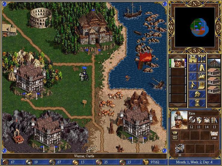
And, surely enough, found the section for the world tiles! (the bg folder in the zip file). Of course, these are commercial assets so I can only use them for testing things out, but they are perfect for that, as I wanted to go for that art style anyway.
So, each terrain type has a bunch of 32x32 images that represent the terrain in its entirety, or transition tiles. I was too lazy to search online if there's any rhyme or reason to the naming of those files, so I did the natural thing: run some batched image processing using ImageMagick to identify the tileable images.
Step 1: Find out the seamless tiles in all directions
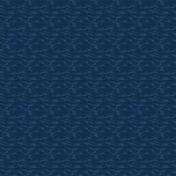
To find out which images tile with themselves, I ran a tiling scipt. A python call for imagemagick commandline looks like this:
"magick montage {}-geometry +0+0 {}".format( (file_in + " ") * numrepeats * numrepeats, file_out)where file_in is the input 32x32 file, file_out is the output tiled file, and numrepeats is the number of tile repeats in each axis.
Results look like this:
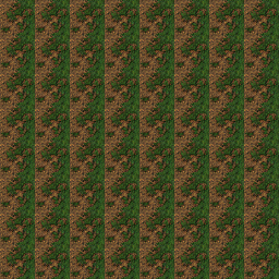
So, great, now I have a list of tiles that are seamless with themselves. But, would they be seamless with other tiles?
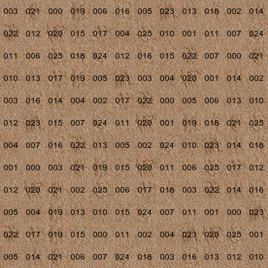
Step 2: Add labels to tiles
Files are of the form "watrtl14.png", "tgrd023.png", etc. So, a prefix for the terrain type, and a number of the id. So, next step is to create images with a label in the middle of the image displaying the tile id:
"magick convert {} -gravity center -annotate +0+0 {} {}".format(file, label, file_out)Result is like this:
![]()
Step 3: Montage of different, labeled tiles
So now here comes the fun part. As we have a version of all the images labeled, I run a montage again as in step 1, but with the following changes:
- Use the labeled images as the base tiles
- If we have 20 images for a terrain, I sample from this set randomly to populate a 12x12 tile grid. This will show what doesn't match with what else! Here's an example

Step 4: Assemble the texture array
Now I select which image set will be used for which biome, e.g. the water images are used for the water biomes (4 of them), by creating variants that are slightly processed in terms of histogram/levels. For each biome, I select a random subset of 16 images. As I have 16 biomes, I end up with 256 image.
So, after a bit of work, the resulting texture looks like this:
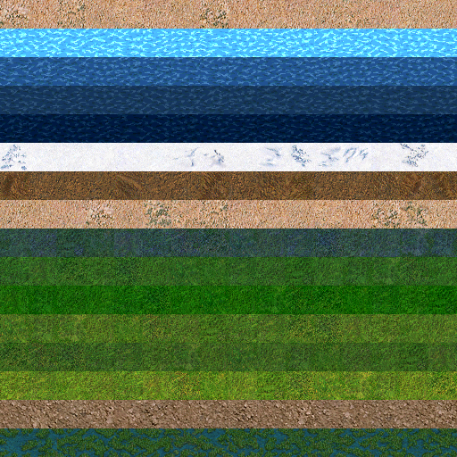
Well, in reality I'm using a source image of 32x8192 which gets interpreted as a texture array of 256 slices, so that I don't have to write manual code for correct mipmapping in the texture atlas. From a quick performance test, there didn't seem to be much difference.
So that's all for how we create the detail texture atlas! Now onto applying it. There's not much to write about how to apply it, as I'm just sampling the texture instead of using a constant color. So, here's a before/after comparison:

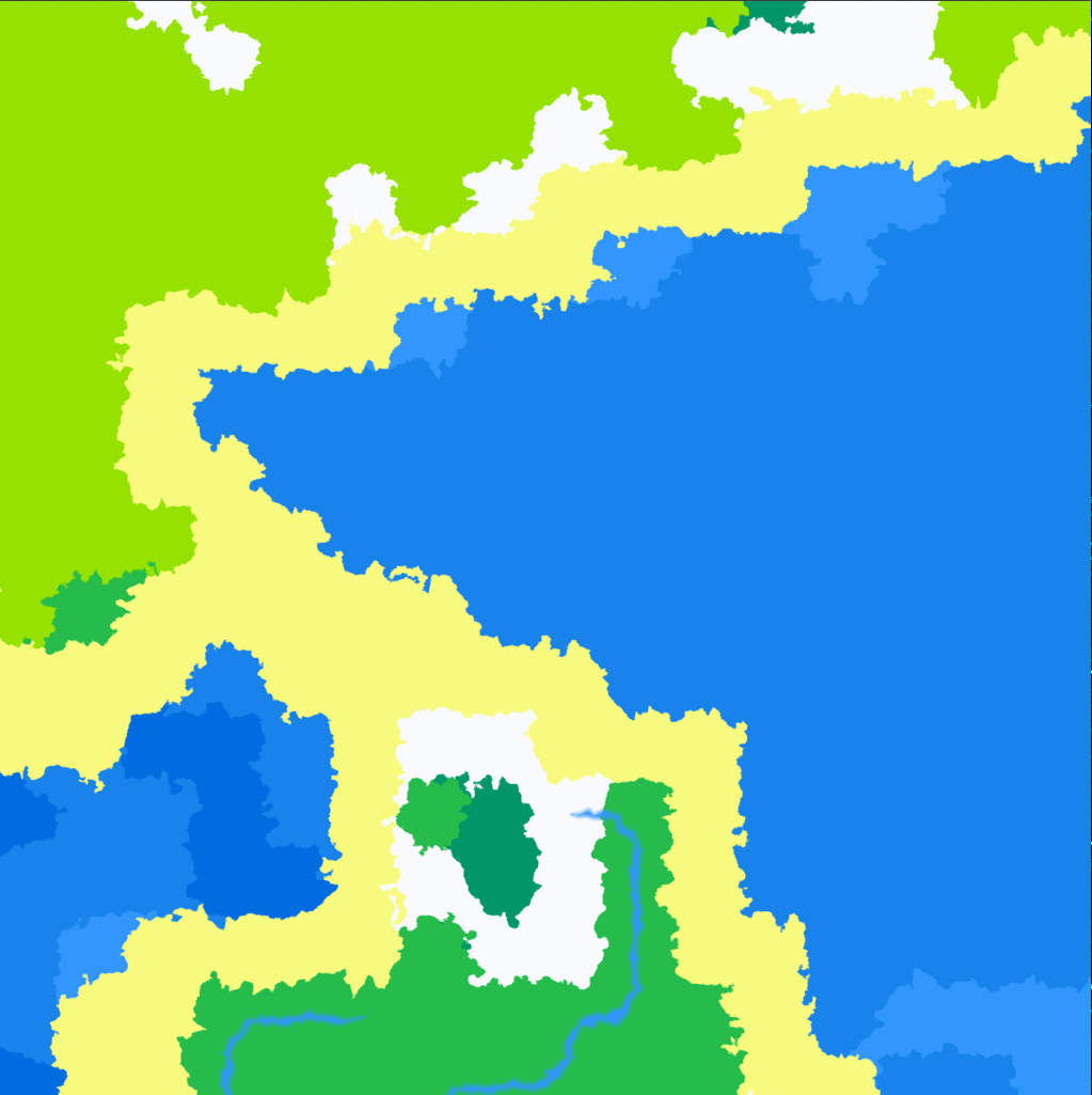

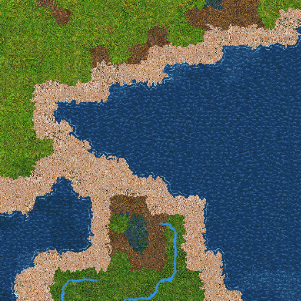
For the observant readers: there's some slight artifact at the tile borders in the above images (and the video below) - this was some incorrect fract() operator on the UV coordinates, this has now been fixed. Here's the associated video in all its animated glory:
The video shows before-and-after the detail textures, the coastal animation, scrolling and zooming in/out on the map. For zoom in/out, I'm using texture filtering like this:
- min filter: linear mipmap linear (to prevent noise at zoomed out level)
- mag filter: nearest (I still want it to look pixely when you zoom in)
- wrap mode: repeat ( it's a texture array, so the filtering is taken care of automatically)
Nevertheless, I found some other resource for future reference for manual filtering/mipmapping if at some point I have to use a regular atlas rather than a texture array.
Coastal waves animation
So that's a nice-looking gimmick, but I'm going to write a bit about how it was implemented anyway.
Remember, instead of storing bitmasks for the biome transitions, we're storing distance fields to the boundary. When rendering, I process the layers one by one, and I'm blending the biome colours. It helps that the seacoast is biome type 0 and the water biomes are types 1,2,3 or 4. So, if there's coast, it will always be the biome type in layer index 0. And if there's water, it will be right after. So, I need the following conditions to be true:
- current layer is a water layer
- first layer is coast
- pixel distance field value from boundary of current layer is negative (pixel is within the mask, ie. our "current" biome)
We need to have recorded the distance field value of the biome in layer index 1, regardless of the layer we're on. This ensures that this is the distance of the first water layer to the coast, which is what we need (the "to the coast" is the crucial bit, as the distance field records values against the previous layer, and we don't want abyssal sea distance to deep sea, if coast, deep sea and abyssal sea are layers on the same tile)
So, now that we have these, we need to compute the waves. For the waves, I'll let code do the talking, as it is noise, domain warping, and the usual:
float t = g_TotalTime*3;
t += 4.1*( snoise2(var_actual_pos*1)*0.5 + 0.5);
float cmpDist = 0.45 + 0.02*(sin(t)*0.5 + 0.5);
cmpDist = 0.41;
if ( layer1dist > cmpDist)
{
    vec3 coastal_water_color = vec3(0.7,0.95,1.0);

    // Put crests at certain distances
    float distFromBoundary = layer1dist;
    float phase = -0.5*t + 2.0*( snoise2(var_actual_pos*10)*0.5 + 0.5) ;
    float dmin = cmpDist;
    float dmax = 0.5;
    float dn = (clamp(distFromBoundary,dmin,dmax) - dmin) / (dmax-dmin);
    float mixFactor = pow( sin(phase + dn*11.0)*0.5 + 0.5, 4.0); // sharpen the result with pow. adjust the phase with time
    mixFactor *= smoothstep( -0.4, 0.4, snoise3( vec3(var_actual_pos*2.0 + vec2(1000),t*0.05)));

    mixFactor *= dn; // smoothly fade out the wave at the boundary distance
    curcolor.xyz = mix( curcolor.xyz, coastal_water_color.xyz, mixFactor);
}
On note about the cmpDist variable. 0.5 is exactly at the boundary ( I encode a signed distance field in [0,1]), and a value slightly away from the coast would be around 0.45.
Next time I'll try my luck with prop placement, and I'll see if I can extract any sample props from that HoMM resource again for test use. But I might actually stop soon with the art, as I think now it should be good enough.